How to Do Exploratory Factor Analysis in SPSS
Knowing how to do exploratory factor analysis in SPSS is essential when you are working with scales, questionnaires, survey items, or multiple observed variables that may reflect a smaller number of underlying constructs. In many research projects, the data do not begin as neat, validated dimensions. Researchers often start with a set of items and need to determine whether those items cluster into meaningful factors. Exploratory factor analysis helps uncover that structure by showing how variables group together, how many factors may exist, and whether the items appear to measure the same latent ideas. UCLA’s SPSS seminar describes EFA as part of identifying latent structure, while the competitor pages consistently present it as a core method for data reduction and construct exploration.
This matters in dissertations, theses, assignments, and journal-style projects because a weak factor structure can affect the validity of later analyses. If the wrong items are grouped together, or if several items load poorly, the interpretation of the scale becomes weaker. That is why EFA is often used before reliability analysis, regression, structural modeling, or broader hypothesis testing. If you need help with scale validation, results writing, or full SPSS analysis, you can also visit SPSS dissertation help, research statistics help, or Request Quotes Now.
What Exploratory Factor Analysis Means
Exploratory factor analysis is a method used to examine whether a set of observed variables can be explained by a smaller number of underlying factors. The purpose is not simply to summarize items, but to identify patterns of shared variance that suggest latent constructs. UCLA’s seminar emphasizes that EFA belongs to the family of latent-variable approaches and that it differs conceptually from principal components analysis because factor analysis focuses on shared variance rather than total variance alone. The SPSS-focused competitor pages describe EFA in simpler terms as a technique for reducing dimensions and discovering the hidden structure of data.
In practice, this means EFA helps answer questions such as these:
| Research question | How EFA helps |
|---|---|
| Do these survey items reflect one construct or several? | Identifies likely factor structure |
| Which items belong together? | Shows item loadings on factors |
| Are some items weak or unsuitable? | Reveals low loadings or cross-loadings |
| Can a long questionnaire be simplified? | Supports item reduction and scale refinement |
That is why EFA is especially common in psychology, education, nursing, management, and social science research using multi-item measures. The SAGE chapter and UCLA materials both frame EFA as a tool for discovering latent structure and reducing complex sets of measured variables into interpretable factors.
When to Use Exploratory Factor Analysis in SPSS
EFA is most useful when the factor structure is not fully established or when you want to examine whether your items behave as expected in your own sample. Competitor pages also repeatedly position EFA as an early-stage tool, with confirmatory factor analysis used later when a researcher wants to test a predefined structure.
You would usually use EFA when:
| Situation | Why EFA is appropriate |
|---|---|
| You created a new questionnaire | Structure is not yet confirmed |
| You adapted items from another study | Structure may differ in your sample |
| You have many related variables | EFA can identify smaller latent dimensions |
| You are validating a scale | EFA helps test whether items cluster logically |
| You want to reduce items before later analysis | EFA supports item screening |
If the structure is already firmly specified and you want to test how well the data fit that known model, confirmatory factor analysis is usually more appropriate. UCLA and the competitor SPSS sites make this distinction clearly.
EFA vs PCA in SPSS
One reason many student reports become weak is that they treat principal components analysis and exploratory factor analysis as the same thing. UCLA’s seminar explains that they are related but not identical. PCA analyzes total variance for dimension reduction, while common factor analysis focuses on shared variance in order to model latent factors. That distinction matters if your goal is scale development, construct validity, or latent interpretation rather than simple data reduction.
Table 1. Difference Between PCA and EFA
| Method | Main purpose | Variance basis | Best use |
|---|---|---|---|
| PCA | Data reduction | Total variance | Reducing variables |
| EFA | Latent structure discovery | Shared/common variance | Identifying constructs |
A strong blog page should address this directly because many competing tutorials move too quickly from the menu path to the output without clarifying the conceptual difference. UCLA’s material is especially useful on this point.
Main Outputs You Need to Understand in SPSS
Most of the competitor pages cover similar SPSS output sections. The difference is usually depth. A better article explains not only what the tables are called, but what they mean and how to write them up. Across the sources you listed, the most important EFA outputs are KMO, Bartlett’s test, communalities, total variance explained, scree plot, and the rotated factor matrix.
Table 2. Core EFA Outputs in SPSS
| Output | What it tells you |
|---|---|
| KMO | Sampling adequacy |
| Bartlett’s test | Whether correlations are sufficient for factor analysis |
| Communalities | How much of each item’s variance is explained by the factors |
| Total variance explained | How much variance is captured by extracted factors |
| Scree plot | Helps judge number of factors |
| Rotated factor matrix | Shows which items load on which factors |
What KMO Means
The Kaiser-Meyer-Olkin measure tests whether the data are suitable for factor analysis. The competitor pages consistently treat it as one of the first outputs to inspect, and UCLA also frames preliminary suitability checks as part of good factor-analytic practice.
Table 3. Common KMO Interpretation Guide
| KMO value | Interpretation |
|---|---|
| .90 and above | Excellent |
| .80 to .89 | Very good |
| .70 to .79 | Good |
| .60 to .69 | Acceptable |
| .50 to .59 | Weak but sometimes tolerated |
| Below .50 | Usually unsuitable |
A higher KMO suggests the correlations among items are compact enough for factor analysis to produce meaningful factors.
What Bartlett’s Test Means
Bartlett’s test of sphericity checks whether the correlation matrix differs significantly from an identity matrix. In plain terms, it tests whether the variables are correlated enough to justify factor analysis. The SPSS tutorials you cited consistently treat a significant Bartlett’s test as supportive of EFA.
A significant result, typically p < .05, suggests that factor analysis is appropriate.
Step-by-Step: How to Do Exploratory Factor Analysis in SPSS
Step 1: Prepare the Items
Before running EFA, make sure the items are coded consistently. Reverse-coded items should already be corrected if the scale requires that. Missing values and obvious data-entry issues should also be reviewed first. A clean factor analysis starts with clean data.
Step 2: Open the Factor Analysis Window
In SPSS, go to:
Analyze → Dimension Reduction → Factor
This is the same menu path described across the SPSS tutorials you listed.
Move the relevant questionnaire items into the variables box.
Step 3: Choose Descriptives and Suitability Checks
Request outputs such as KMO and Bartlett’s test and the correlation matrix if needed. These help you judge whether EFA should proceed.
Step 4: Select the Extraction Method
This is where many student reports need more precision. UCLA emphasizes that extraction matters conceptually, and that principal axis factoring and maximum likelihood are common factor-analysis approaches, while principal components is different in aim.
If your goal is true exploratory factor analysis for latent constructs, principal axis factoring is often more defensible than simply defaulting to principal components.
Step 5: Decide How Many Factors to Retain
Common factor-retention tools include:
| Criterion | What it does |
|---|---|
| Eigenvalues greater than 1 | Common but imperfect rule |
| Scree plot | Helps identify the point where the curve levels off |
| Theory | Keeps retained factors conceptually meaningful |
| Interpretability | Factors should make practical sense |
UCLA’s seminar and the SPSS tutorials both discuss extraction and interpretation, while many competitor pages lean heavily on eigenvalues and scree plot.
Step 6: Choose Rotation
Rotation helps produce a clearer and more interpretable factor solution. UCLA explains that after extraction, rotation is used to obtain a more interpretable solution.
Table 4. Common Rotation Choices
| Rotation type | When it is used |
|---|---|
| Varimax | When factors are treated as uncorrelated |
| Oblimin / Promax | When factors may be correlated |
A better blog page should explain that social science constructs often do correlate, so an oblique rotation may sometimes be more realistic than always choosing varimax.
Step 7: Run the Analysis and Inspect the Output
After choosing extraction and rotation, run the model and move carefully through the key outputs. Do not jump straight to the rotated matrix without checking whether the data were suitable in the first place.
How to Interpret the Key EFA Tables in SPSS
KMO and Bartlett’s Test Table
Table 5. Example KMO and Bartlett’s Test
| Statistic | Value |
|---|---|
| KMO | .84 |
| Bartlett’s Test Chi-square | 612.47 |
| df | 105 |
| p | < .001 |
Interpretation
The KMO value of .84 indicates very good sampling adequacy, and Bartlett’s test was statistically significant, suggesting that the correlation matrix was suitable for exploratory factor analysis.
That type of sentence is stronger than simply saying “the assumptions were met,” because it names the evidence directly.
Communalities Table
Communalities show how much of each item’s variance is explained by the retained factors. Items with very low communalities may not fit the factor structure well.
Table 6. Example Communalities
| Item | Extraction communality |
|---|---|
| Item 1 | .63 |
| Item 2 | .71 |
| Item 3 | .58 |
| Item 4 | .29 |
| Item 5 | .67 |
Interpretation
Most items showed acceptable communalities, but Item 4 had a relatively low extracted communality of .29, suggesting that it was not well explained by the retained factors.
That kind of wording gives the reader a reasoned interpretation rather than a list of numbers.
Total Variance Explained Table
This table shows how much variance is explained by the extracted factors. Competitor tutorials commonly discuss this table, but stronger writing explains why it matters.
Table 7. Example Total Variance Explained
| Factor | Eigenvalue | % Variance | Cumulative % |
|---|---|---|---|
| 1 | 4.62 | 30.80 | 30.80 |
| 2 | 2.11 | 14.07 | 44.87 |
| 3 | 1.46 | 9.73 | 54.60 |
Interpretation
Three factors were retained, together accounting for 54.60% of the total variance. The first factor explained the largest proportion of variance, followed by the second and third factors.
Scree Plot
The scree plot helps identify where the curve begins to level off. UCLA’s materials emphasize extraction and the judgment involved in determining the best factor structure, not simply following one mechanical rule.
In a strong write-up, you can note that the scree plot supported the retained factor solution rather than relying only on eigenvalues.
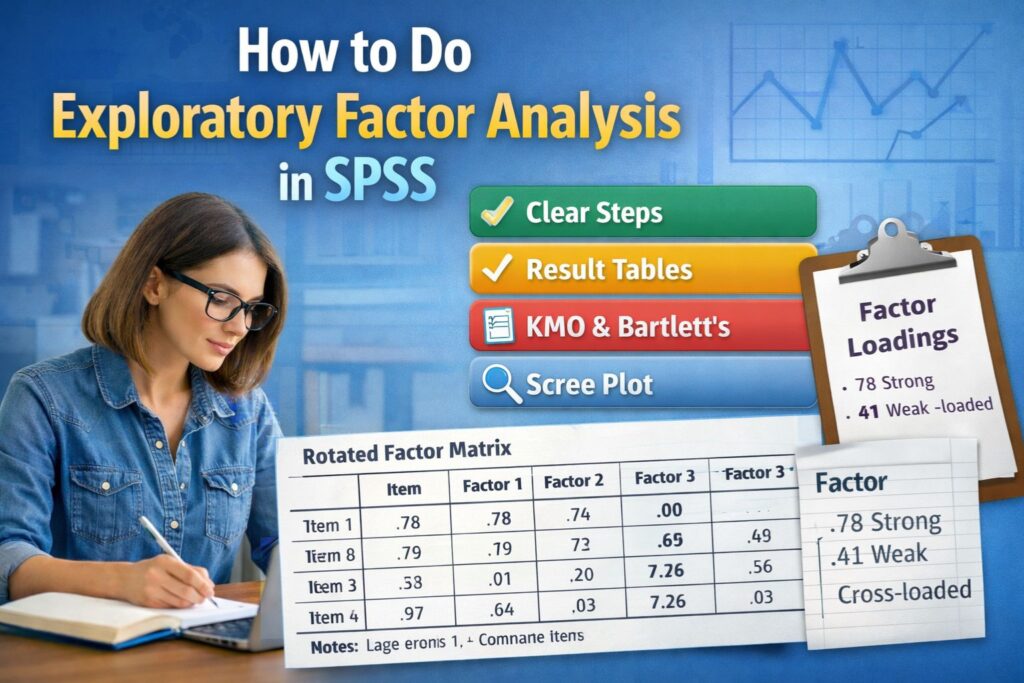
Rotated Factor Matrix
The rotated factor matrix is usually the most important table for interpretation because it shows which items load on which factors. Competitor pages consistently center this table in EFA interpretation.
Table 8. Example Rotated Factor Matrix
| Item | Factor 1 | Factor 2 | Factor 3 |
|---|---|---|---|
| Item 1 | .78 | .14 | .10 |
| Item 2 | .74 | .19 | .08 |
| Item 3 | .69 | .23 | .12 |
| Item 4 | .11 | .81 | .09 |
| Item 5 | .18 | .76 | .16 |
| Item 6 | .22 | .12 | .73 |
| Item 7 | .17 | .08 | .70 |
| Item 8 | .44 | .41 | .09 |
Interpretation
Items 1 to 3 loaded strongly on Factor 1, Items 4 and 5 loaded on Factor 2, and Items 6 and 7 loaded on Factor 3. Item 8 showed cross-loadings on Factors 1 and 2, suggesting that it may not belong clearly to a single factor and may require closer review.
That final sentence is where many shorter competitor posts stop too early. A stronger page should teach readers how to spot a problematic item.
How to Judge Factor Loadings
The exact cutoff depends on sample size, research area, and reporting convention, but many student projects treat loadings around .40 or above as meaningfully interpretable.
Table 9. Practical Guide to Factor Loadings
| Loading size | Practical meaning |
|---|---|
| .30 to .39 | Weak to modest |
| .40 to .49 | Acceptable |
| .50 to .69 | Good |
| .70 and above | Strong |
What matters most is not just whether an item loads above a threshold, but whether it loads clearly on one factor and not strongly on several.
What to Do With Cross-Loadings
A cross-loading happens when an item loads meaningfully on more than one factor. This makes interpretation weaker because the item is not clearly representing a single construct.
Common responses to cross-loading items
| Action | When it may help |
|---|---|
| Remove the item | If it weakens conceptual clarity |
| Retain with caution | If theory strongly supports it |
| Re-run the model | If several items were removed |
| Review wording | If the item may be ambiguous |
A stronger EFA page should not pretend every item fits neatly. Real data often contain items that need revision or removal.
How to Name the Factors
Factor naming should be based on the shared content of the items loading on each factor. You do not name a factor based only on the highest loading item. You name it based on the conceptual meaning of the group of items.
Example
| Factor | Main item themes | Possible label |
|---|---|---|
| Factor 1 | Confidence, capability, persistence | Self-efficacy |
| Factor 2 | Anxiety, fear, tension | Psychological distress |
| Factor 3 | Planning, organization, structure | Self-management |
Good factor names make the findings easier to understand and easier to defend in discussion and conclusion sections.
Sample Results Paragraph for a Dissertation or Thesis
Exploratory factor analysis using principal axis factoring with varimax rotation was conducted on the 15 questionnaire items. The data were suitable for factor analysis, as the Kaiser-Meyer-Olkin measure of sampling adequacy was .84 and Bartlett’s test of sphericity was statistically significant, χ²(105) = 612.47, p < .001. Three factors with eigenvalues greater than 1 were retained, accounting for 54.60% of the total variance. The rotated factor matrix showed that Items 1 to 3 loaded strongly on Factor 1, Items 4 and 5 loaded on Factor 2, and Items 6 and 7 loaded on Factor 3. One item showed cross-loadings and was reviewed carefully before final interpretation.
That paragraph is stronger than many competitor examples because it combines suitability, extraction result, retained factors, explained variance, and factor-pattern interpretation in one clean section.
Best Table Format for Reporting EFA Results
Table 10. Summary of Exploratory Factor Analysis Results
| Item | Factor loading | Assigned factor | Decision |
|---|---|---|---|
| Item 1 | .78 | Factor 1 | Retained |
| Item 2 | .74 | Factor 1 | Retained |
| Item 3 | .69 | Factor 1 | Retained |
| Item 4 | .81 | Factor 2 | Retained |
| Item 5 | .76 | Factor 2 | Retained |
| Item 6 | .73 | Factor 3 | Retained |
| Item 7 | .70 | Factor 3 | Retained |
| Item 8 | .44 / .41 | Cross-loaded | Reviewed |
This kind of table works very well in dissertations and thesis chapters because it gives the reader a clean summary without forcing them to scan a dense software output table.
Common Mistakes When Doing Exploratory Factor Analysis in SPSS
Treating PCA as Identical to EFA
UCLA clearly distinguishes the two, and that distinction matters for construct-based interpretation.
Ignoring KMO and Bartlett’s Test
A factor solution should not be interpreted before checking whether the data were suitable.
Relying Only on Eigenvalues Greater Than 1
That rule is common, but it should be supported by scree plot judgment and theoretical sense. UCLA’s seminar emphasizes the broader decision process.
Keeping Cross-Loading Items Without Discussion
This weakens the construct interpretation and often leads to examiner comments.
Naming Factors Too Quickly
Factor labels should reflect the meaning of the item set, not just the highest-loading variable.
Copying Raw SPSS Output Into the Results Section
A good results section explains the factor structure clearly rather than reproducing screenshots without interpretation.
EFA and Reliability Analysis
Once factors are identified, the next step often involves checking reliability for each retained factor or subscale. Competitor SPSS sites commonly place EFA and reliability close together because they are often used in the same scale-development workflow.
If you are moving from factor extraction to internal consistency testing, you can continue with reliability analysis help, Cronbach’s alpha in SPSS, or data analysis help. If you want direct support with your own questionnaire, Request Quotes Now.
How to Report EFA in APA-Style Writing
A concise academic sentence often includes the extraction method, rotation method, suitability statistics, number of retained factors, explained variance, and notable loading patterns.
Example APA-style sentence
Exploratory factor analysis using principal axis factoring and varimax rotation indicated a three-factor solution, with KMO = .84 and Bartlett’s test of sphericity significant at p < .001; the retained factors explained 54.60% of the total variance.
That kind of wording is much more effective than simply writing, “EFA was done and three factors were found.”
Final Thoughts
Learning how to do exploratory factor analysis in SPSS is about more than clicking through the software menu. It is about understanding whether the data support factor analysis, selecting an appropriate extraction approach, deciding how many factors to retain, interpreting the rotated matrix carefully, and reporting the results in a way that makes conceptual and statistical sense. The competitor pages you listed cover parts of this process, especially the SPSS steps and basic interpretation, but the strongest research writing comes from combining method choice, clear item screening, cross-loading judgment, and polished results reporting in one coherent explanation.
If you need help validating a scale, refining factors, reporting EFA clearly, or writing the results for your dissertation or thesis, you can explore statistical analysis help, SPSS help for students, or Request Quotes Now.
FAQ
What is exploratory factor analysis in SPSS?
Exploratory factor analysis in SPSS is a method used to identify the underlying factor structure of a set of observed variables, especially when the researcher wants to discover how items cluster into latent constructs. UCLA and the SPSS tutorials you listed all frame EFA as a tool for uncovering latent structure and reducing complexity.
What is the difference between EFA and PCA?
PCA focuses on total variance for data reduction, while EFA focuses on shared variance to identify latent constructs. UCLA’s seminar highlights this distinction directly.
What KMO value is acceptable for factor analysis?
A KMO value of .60 or above is often treated as acceptable, with higher values indicating better sampling adequacy. This is consistent with the way SPSS EFA tutorials use KMO as a suitability check.
Why is Bartlett’s test important in EFA?
Bartlett’s test checks whether the variables are correlated enough for factor analysis. A statistically significant result supports the use of EFA. Competitor tutorials consistently use it for that purpose.
How many factors should I retain in EFA?
Factor retention should consider eigenvalues, scree plot, theory, and interpretability rather than relying on only one rule. UCLA’s materials especially support a more thoughtful retention decision.
What factor loading is considered acceptable?
Many student projects treat .40 or above as acceptable, though the best threshold depends on sample size, field, and the clarity of the overall factor pattern.
What should I do with cross-loading items?
Cross-loading items should be reviewed carefully because they do not represent one factor clearly. Depending on theory and clarity, they may be removed, revised, or retained with caution.
Should I use varimax or oblimin rotation?
Varimax is common when factors are treated as uncorrelated, while oblimin is more suitable when factors may be related. Rotation is used to improve interpretability, as UCLA explains.
Can I use EFA before reliability analysis?
Yes. EFA is often used to identify factor structure before checking reliability for each retained factor or subscale. This workflow is reflected across the SPSS-focused materials reviewed.
How do I report exploratory factor analysis results in SPSS?
A strong report should include the extraction method, rotation method, KMO, Bartlett’s test, number of retained factors, variance explained, and a summary of the factor loadings.