How to Run Regression in Minitab: Step-by-Step Guide for Students and Researchers
Learning how to run regression in Minitab is important for students, researchers, dissertation writers, business analysts, and professionals who need to examine relationships between variables. Minitab makes regression analysis easier to perform, but the real challenge is not just running the model. The harder part is knowing what the output means, whether the assumptions are satisfied, and how to report the findings correctly.
Many people can follow the menu path in Minitab, but they struggle when they see coefficients, p-values, R-squared, adjusted R-squared, residual plots, confidence intervals, and VIF values. This guide explains the full process in a clear and practical way, from preparing your data to interpreting and reporting your regression results.
If you need support beyond this guide, Statistical Analysis Help provides assistance with Minitab, regression analysis, dissertation statistics, data interpretation, and statistical reporting.
What Is Regression Analysis in Minitab?
Regression analysis is a statistical method used to examine the relationship between a response variable and one or more predictor variables. In simple terms, regression helps you understand whether one variable can explain or predict changes in another variable.
The response variable is the outcome you want to predict or explain. The predictor variable is the variable used to explain or predict that outcome.
For example, if a researcher wants to know whether study hours predict exam scores, the exam score is the response variable and study hours is the predictor variable.
If there is only one predictor, the analysis is called simple linear regression. If there are two or more predictors, the analysis is called multiple regression.
Regression can be used in many fields. A business analyst may use it to predict sales revenue. A healthcare researcher may use it to study patient recovery time. A student may use it to test a dissertation hypothesis. A quality improvement professional may use it to understand which process factors affect product defects.
If your project requires choosing the correct model or interpreting regression findings, Regression Analysis Help can help you understand the statistical meaning behind the output.
When Should You Use Regression in Minitab?
You should use regression in Minitab when you want to examine whether one or more variables are related to a numeric outcome. Regression is commonly used when the goal is to predict, explain, or test relationships between variables.
For example, regression may be appropriate if you want to answer questions such as:
- Does study time predict exam performance?
- Do advertising spend and product price predict sales revenue?
- Does patient age predict recovery time?
- Do machine speed and temperature predict defect rates?
- Do employee experience and training hours predict job performance?
In most linear regression models, the response variable should be numeric. Examples include exam score, revenue, blood pressure, customer satisfaction score, production time, employee performance score, or cost.
If your response variable is categorical, such as yes or no, pass or fail, or low, medium, and high, you may need logistic regression or another type of model instead of ordinary linear regression.
Common Types of Regression in Minitab
Minitab supports several regression methods. The right choice depends on your research question and the type of response variable you have.
Simple Linear Regression
Simple linear regression uses one predictor to explain or predict one continuous response variable.
Example:
Study hours predicting exam score.
This model is often used when you want to understand a direct relationship between two variables.
Multiple Linear Regression
Multiple regression uses two or more predictors to explain or predict one continuous response variable.
Example:
Study hours, attendance, and GPA predicting exam score.
Multiple regression is useful because it allows you to examine the effect of each predictor while controlling for the other predictors in the model. If you are working with several predictors, multiple regression analysis help can help with model setup, interpretation, and reporting.
Regression With Categorical Predictors
Minitab can also include categorical predictors in regression models. These are variables that represent groups or categories, such as treatment group, gender, region, department, machine type, or teaching method.
Categorical predictors must be handled correctly. If a categorical variable is mistakenly treated as a continuous number, the model may produce misleading results.
Logistic Regression
Logistic regression is used when the response variable is categorical. Binary logistic regression is used for outcomes with two categories, such as yes or no, pass or fail, or purchased and did not purchase.
Poisson Regression
Poisson regression is used when the response variable is a count, such as number of defects, number of complaints, number of errors, or number of patient visits.
This article focuses mainly on simple linear regression and multiple linear regression because those are the most common models people use when searching for how to run regression in Minitab.
How to Prepare Your Data Before Running Regression in Minitab
Before running regression, your dataset must be organized correctly. Many regression problems happen because the data is not prepared properly.
Each variable should be placed in its own column. Each row should represent one observation. For example, if you are studying student performance, each row may represent one student, while each column may represent exam score, study hours, attendance, and GPA.
Use clear variable names so the output is easy to understand. Names like “Exam Score,” “Study Hours,” “Attendance,” and “Previous GPA” are much better than names like “C1,” “Var2,” or “Data A.”
You should also check for missing values before running the model. Missing values can reduce your sample size because Minitab may exclude incomplete rows from the analysis. If many values are missing, your results may become less reliable.
Outliers should also be reviewed before and after running regression. An outlier is an unusual value that may strongly affect the regression equation. Outliers should not be deleted automatically. Instead, you should investigate whether they are data entry errors, valid extreme observations, or signs that the model does not fit the data well.
You should also check whether the relationship between your predictor and response appears reasonably linear. Scatterplots are useful for this. If the relationship is curved, a simple linear regression model may not be appropriate.
For help preparing, cleaning, and organizing datasets before analysis, visit Data Analysis Help.
How to Run Simple Linear Regression in Minitab
Simple linear regression is used when you have one response variable and one predictor variable.
For example, suppose you want to test whether study hours predict exam score. In this case, exam score is the response variable and study hours is the predictor variable.
To run simple linear regression in Minitab:
Open your dataset in Minitab.
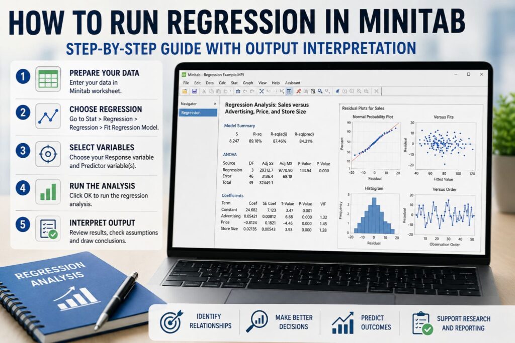
Go to Stat > Regression > Regression > Fit Regression Model.
In the Response box, select the outcome variable. In this example, that would be Exam Score.
In the Continuous predictors box, select the predictor variable. In this example, that would be Study Hours.
Click Graphs and select the residual plots you want Minitab to produce. The four-in-one residual plot is often useful because it gives several diagnostic plots in one view.
Click OK to run the model.
Minitab will produce the regression output, which usually includes the regression equation, model summary, analysis of variance table, coefficients table, p-values, R-squared values, and residual plots.
The most important part is not just running the model. You must also interpret whether study hours significantly predict exam score, how strong the relationship is, and whether the residual plots suggest that the model assumptions are reasonable.
How to Run Multiple Regression in Minitab
Multiple regression is used when you have one response variable and two or more predictor variables.
For example, suppose you want to test whether study hours, attendance, and previous GPA predict exam score. In this case, exam score is the response variable, while study hours, attendance, and previous GPA are the predictor variables.
To run multiple regression in Minitab:
Open your dataset in Minitab.
Go to Stat > Regression > Regression > Fit Regression Model.
In the Response box, select your outcome variable.
In the Continuous predictors box, select all continuous predictor variables.
If your model includes categorical predictors, add them in the categorical predictors section if your version of Minitab provides that option.
Click Graphs and select residual plots.
Click OK.
Minitab will run the multiple regression model and display the output.
Multiple regression is more complex than simple linear regression because each coefficient is interpreted while holding the other predictors constant. For example, if study hours, attendance, and GPA are all included in the model, the coefficient for study hours tells you how exam score changes when study hours increase by one unit, assuming attendance and GPA remain constant.
Using Minitab Assistant for Regression
Some versions of Minitab include an Assistant tool for regression. This can be helpful for beginners because it provides a guided approach to selecting and interpreting regression models.
You may find it under Assistant > Regression.
The Assistant can be useful when you are not sure which regression option to choose. However, the standard Fit Regression Model option usually provides more control. This is often better for dissertations, research papers, class assignments, and professional reports because you can choose your predictors, examine detailed output, check assumptions, and report the results more carefully.
Example of a Regression Dataset in Minitab
Assume a researcher wants to know whether study hours, attendance, and previous GPA predict exam score.
The dataset may include the following variables:
| Student | Exam Score | Study Hours | Attendance | Previous GPA |
|---|---|---|---|---|
| 1 | 78 | 5 | 86 | 3.1 |
| 2 | 85 | 7 | 92 | 3.4 |
| 3 | 69 | 3 | 75 | 2.8 |
| 4 | 91 | 9 | 96 | 3.8 |
| 5 | 74 | 4 | 81 | 3.0 |
| 6 | 88 | 8 | 94 | 3.6 |
| 7 | 72 | 4 | 78 | 2.9 |
| 8 | 95 | 10 | 98 | 3.9 |
In this example, Exam Score is the response variable. Study Hours, Attendance, and Previous GPA are predictor variables.
A multiple regression model would estimate how well these predictors explain differences in exam scores.
How to Interpret Minitab Regression Output
After running regression in Minitab, the output may seem overwhelming at first. The best approach is to interpret it in a logical order.
Start with the overall model. Check whether the model is statistically significant. Then review R-squared and adjusted R-squared to understand how much variation the model explains. Next, examine the coefficients table to see which predictors are statistically significant and how each predictor is related to the response variable. Finally, check residual plots and assumption diagnostics.
Regression Equation
The regression equation shows the predicted relationship between the response variable and the predictor variables.
A simple regression equation may look like this:
Predicted Exam Score = 60 + 3.5 Study Hours
This means each additional study hour is associated with a 3.5 point increase in predicted exam score.
A multiple regression equation may look like this:
Predicted Exam Score = 25 + 2.1 Study Hours + 0.35 Attendance + 6.2 Previous GPA
This means the predicted exam score is based on study hours, attendance, and previous GPA together.
Coefficients
The coefficient tells you how much the response variable is expected to change when the predictor increases by one unit, assuming the other variables remain constant.
For example, if the coefficient for study hours is 2.1, each additional study hour is associated with a 2.1 point increase in predicted exam score, assuming attendance and GPA stay the same.
P-Values
The p-value helps determine whether a predictor is statistically significant. A common cutoff is 0.05. If the p-value is less than 0.05, the predictor is often considered statistically significant.
However, p-values should not be interpreted alone. You should also consider the size of the coefficient, confidence intervals, sample size, research question, and model assumptions.
R-Squared
R-squared tells you how much variation in the response variable is explained by the model.
For example, if R-squared is 72 percent, the model explains 72 percent of the variation in the response variable.
A high R-squared can be useful, but it does not automatically mean the model is correct. A model can have a high R-squared and still violate important assumptions.
Adjusted R-Squared
Adjusted R-squared is especially useful in multiple regression. It adjusts for the number of predictors in the model.
This matters because regular R-squared usually increases when more predictors are added, even if those predictors do not truly improve the model. Adjusted R-squared gives a more balanced view.
Predicted R-Squared
Predicted R-squared shows how well the model may perform when predicting new data. If predicted R-squared is much lower than R-squared, the model may be overfitting the sample data.
Analysis of Variance Table
The analysis of variance table tests whether the overall regression model is statistically significant. It usually includes the F-value and the model p-value.
If the overall model p-value is less than 0.05, the model is often considered statistically significant.
Residual Plots
Residual plots help you check whether the model assumptions are reasonable. They are important because regression output can look statistically significant even when the model does not fit the data well.
How to Interpret the Regression Equation
The regression equation allows you to estimate the predicted value of the response variable.
For multiple regression, the equation may be written as:
Predicted Score = b0 + b1 Study Hours + b2 Attendance + b3 GPA
In this equation, b0 is the intercept. The values b1, b2, and b3 are coefficients for the predictors.
Suppose Minitab gives this equation:
Predicted Score = 25 + 2.1 Study Hours + 0.35 Attendance + 6.2 GPA
This means:
For each additional study hour, the predicted score increases by 2.1 points, holding attendance and GPA constant.
For each one-point increase in attendance, the predicted score increases by 0.35 points, holding study hours and GPA constant.
For each one-point increase in GPA, the predicted score increases by 6.2 points, holding study hours and attendance constant.
When writing the results, be careful with causal language. Unless the study design supports causation, it is better to say “is associated with,” “predicts,” or “is related to” instead of saying “causes.”
How to Check Regression Assumptions in Minitab
Regression assumptions help determine whether your results are reliable. A model can produce p-values and coefficients even when assumptions are not satisfied, so assumption checking is an important part of the analysis.
The main assumptions include linearity, independence, normality of residuals, constant variance, no major outliers, and no serious multicollinearity.
Linearity
Linearity means the relationship between the predictor and response should be approximately straight. You can check this using scatterplots and residual plots.
If the residuals show a curved pattern, the relationship may not be linear. In that case, you may need a transformation, polynomial term, or a different model.
Independence
Independence means each observation should be independent of the others. This is especially important when data is collected over time or from repeated measurements.
The residuals versus order plot can help identify time-related patterns. If the plot shows a trend or cycle, the independence assumption may be questionable.
Normality of Residuals
Regression does not require every raw variable to be normally distributed, but the residuals should be approximately normal for many regression tests and confidence intervals.
You can check this using the normal probability plot and histogram of residuals. If the residuals are strongly skewed or show major departures from normality, the model may need further review.
Constant Variance
Constant variance means the spread of residuals should be similar across fitted values. You can check this using the residuals versus fits plot.
If the plot shows a funnel shape, the model may have unequal variance. This can affect standard errors, p-values, and confidence intervals.
Outliers and Influential Observations
Outliers are unusual values that can strongly affect the regression line. Minitab may flag unusual observations in the output.
Do not remove outliers without a valid reason. Investigate whether the values are data entry errors, valid extreme cases, or evidence that the model does not fit the data well.
Multicollinearity
Multicollinearity occurs when predictor variables are highly related to each other. This is mainly an issue in multiple regression.
Minitab can report VIF values to help identify multicollinearity. High VIF values may suggest that some predictors overlap too much, making coefficients unstable or difficult to interpret.
How to Read Minitab Residual Plots
Residual plots are one of the most important parts of regression diagnostics. They help show whether the model fits the data appropriately.
Normal Probability Plot
The normal probability plot checks whether residuals are approximately normal. A good plot usually has points that fall close to a straight line.
If the points show a strong curve, an S-shaped pattern, or extreme departures from the line, the residuals may not be normally distributed.
Histogram of Residuals
The histogram shows the shape of the residual distribution. A reasonable histogram is often roughly bell-shaped, although small samples may not look perfect.
Strong skew, multiple peaks, or extreme values may indicate a problem.
Residuals Versus Fits Plot
The residuals versus fits plot helps check linearity and constant variance. A good plot usually shows random scatter around zero.
A curved pattern may suggest nonlinearity. A funnel shape may suggest unequal variance. Clusters or extreme points may suggest outliers or missing variables.
Residuals Versus Order Plot
The residuals versus order plot helps check whether residuals follow a time-related pattern. A good plot should look random.
A trend, cycle, or long run of points above or below zero may suggest that observations are not independent.
How to Check Multicollinearity With VIF in Minitab
VIF stands for variance inflation factor. It helps determine whether predictors in a multiple regression model are too strongly related to each other.
A VIF close to 1 usually suggests low multicollinearity. Values between 2 and 5 may suggest moderate overlap. Values above 5 may be a concern, and values above 10 are often treated as serious multicollinearity.
These are general guidelines, not absolute rules. The seriousness of multicollinearity depends on the field, sample size, research question, and purpose of the model.
If VIF is high, you may need to remove one of the overlapping predictors, combine similar variables, use theory to decide which predictor is more important, or run separate models.
How to Use Minitab Regression for Prediction
Regression can be used to estimate predicted values.
Suppose the regression equation is:
Predicted Exam Score = 25 + 2.1 Study Hours + 0.35 Attendance + 6.2 GPA
If a student studied for 8 hours, had 90 percent attendance, and had a GPA of 3.5, the predicted score would be:
25 + 2.1(8) + 0.35(90) + 6.2(3.5)
25 + 16.8 + 31.5 + 21.7 = 95
The predicted exam score is 95.
It is also important to understand the difference between a confidence interval and a prediction interval. A confidence interval estimates the average response for similar cases. A prediction interval estimates the likely range for one individual case. Prediction intervals are usually wider because individual outcomes are harder to predict.
How to Report Regression Results From Minitab
A strong regression report should include the purpose of the analysis, the response variable, the predictor variables, the overall model result, R-squared values, coefficients, p-values, confidence intervals, assumption checks, and a clear interpretation.
For dissertation or thesis support, Dissertation Statistics Help can help with statistical write-ups, results chapters, and interpretation.
Simple Linear Regression Reporting Example
A simple linear regression was conducted to determine whether study hours predicted exam score. The overall regression model was statistically significant, F(df1, df2) = [value], p = [value], indicating that study hours significantly predicted exam score. The model explained [R-squared percent] of the variance in exam score. The coefficient for study hours was positive and statistically significant, b = [coefficient], p = [value], suggesting that higher study hours were associated with higher predicted exam scores.
Multiple Regression Reporting Example
A multiple regression analysis was conducted to examine whether study hours, attendance, and previous GPA predicted exam score. The overall model was statistically significant, F(df1, df2) = [value], p = [value], and explained [R-squared percent] of the variance in exam score, with an adjusted R-squared of [value]. Study hours was a statistically significant predictor, b = [coefficient], p = [value]. Attendance was also statistically significant, b = [coefficient], p = [value]. Previous GPA was not statistically significant, p = [value]. These results suggest that study hours and attendance were associated with exam score after controlling for the other predictors in the model.
Dissertation Results Paragraph Example
To test the relationship between the predictor variables and the outcome variable, a multiple regression analysis was conducted in Minitab. The assumptions of regression were evaluated using residual plots, normal probability plots, and multicollinearity diagnostics. The overall model was statistically significant, F(df1, df2) = [value], p = [value], indicating that the predictors collectively explained a significant proportion of variance in the outcome variable. The model explained [R-squared percent] of the variance, with an adjusted R-squared of [value]. The coefficients indicated that [insert significant predictors] were statistically significant predictors of [response variable]. Therefore, the findings [supported or did not support] the research hypothesis.
Common Mistakes When Running Regression in Minitab
One common mistake is selecting the wrong response variable. The response variable should be the outcome you want to predict or explain. If you place the predictor in the response field, the model will answer the wrong question.
Another mistake is ignoring residual plots. A model can have significant p-values but still show poor residual patterns. Residual plots help identify nonlinearity, unequal variance, outliers, and independence problems.
Many users also report only R-squared. R-squared is useful, but it is not enough. A complete regression interpretation should include coefficients, p-values, confidence intervals, adjusted R-squared, residual plots, and assumption checks.
Another common problem is overclaiming causation. Regression can show association, but it does not automatically prove that one variable causes another. Unless the study design supports causal inference, use careful wording.
Users also make mistakes with categorical variables. If categorical predictors are coded as numbers, they should not automatically be treated as continuous variables. Make sure they are entered correctly.
Troubleshooting Minitab Regression Problems
If your predictor does not appear in the regression dialog box, check whether the variable type is correct and whether there are missing or invalid values.
If your p-values are not significant, it may mean the relationship is weak, the sample size is small, the predictors overlap, or the model does not match the research question.
If R-squared is low, the predictors may not explain much of the outcome. A low R-squared does not always mean the model is useless, but it should be interpreted carefully.
If residual plots look poor, the model assumptions may not be satisfied. You may need to transform a variable, add a missing predictor, use a different model, or investigate outliers.
If VIF values are high, the predictors may be too strongly related to each other. You may need to remove or combine predictors.
If your output is confusing, review the research question first. A clear research question makes it easier to identify the correct response variable, predictors, model type, and interpretation.
Minitab Regression Output Checklist
Before finalizing your regression results, make sure you have reviewed the full output carefully.
Confirm that the response variable is correct.
Confirm that the predictor variables are correct.
Check whether the overall model is statistically significant.
Review the coefficient for each predictor.
Check p-values and confidence intervals.
Review R-squared, adjusted R-squared, and predicted R-squared.
Inspect the residual plots.
Check VIF values if running multiple regression.
Write the regression equation correctly.
Interpret results in the context of the research question.
Avoid unsupported causal claims.
Report assumption checks clearly.
This checklist helps ensure that your interpretation is complete and not based on one statistic alone.
When to Get Help With Regression in Minitab
You may need help with Minitab regression if you are unsure which model to use, how to prepare your dataset, how to check assumptions, or how to explain the output in a professional format.
Students and researchers often seek help when their Minitab output is confusing, their residual plots look unusual, their p-values are not significant, their VIF values are high, or their professor or committee asks them to revise the analysis.
You may also need help if you are writing a dissertation, preparing a results chapter, responding to reviewer feedback, or working with a tight deadline.
At Statistical Analysis Help, we help students, researchers, and professionals with regression analysis, Minitab output interpretation, dissertation statistics, data analysis, and statistical reporting.
If you are unsure whether your regression model is correct or need help interpreting your Minitab output, you can Request a Quote Now for expert support.
Frequently Asked Questions About Regression in Minitab
How do I run simple linear regression in Minitab?
To run simple linear regression in Minitab, go to Stat > Regression > Regression > Fit Regression Model. Select your outcome variable in the response field and your predictor variable in the continuous predictors field. Then choose residual plots and click OK.
How do I run multiple regression in Minitab?
To run multiple regression in Minitab, use Stat > Regression > Regression > Fit Regression Model. Select one response variable and add two or more predictors. If you have categorical predictors, enter them in the appropriate categorical predictors section.
How do I interpret regression output in Minitab?
Start with the regression equation, model summary, ANOVA table, coefficients table, p-values, R-squared values, and residual plots. The coefficients explain the direction and size of the relationship. The p-values help identify statistically significant predictors. The residual plots help check assumptions.
What does R-squared mean in Minitab regression?
R-squared shows the percentage of variation in the response variable explained by the model. For example, an R-squared of 70 percent means the model explains 70 percent of the variation in the response variable.
What is adjusted R-squared in Minitab?
Adjusted R-squared adjusts R-squared based on the number of predictors in the model. It is especially useful in multiple regression because it helps prevent overvaluing models that include unnecessary predictors.
How do I check regression assumptions in Minitab?
You can check regression assumptions using residual plots, scatterplots, normal probability plots, histograms, residuals versus fits plots, residuals versus order plots, and VIF values. These help evaluate linearity, normality of residuals, constant variance, independence, outliers, and multicollinearity.
What are residual plots in Minitab?
Residual plots show the differences between actual and predicted values. They help you determine whether the regression model fits the data well and whether assumptions are reasonable.
Can Minitab run logistic regression?
Yes. Minitab can run logistic regression. Logistic regression is used when the response variable is categorical, such as yes or no, pass or fail, or purchased and did not purchase.
When should I get help with Minitab regression?
You should consider getting help if you are unsure which model to use, your residual plots look problematic, your VIF values are high, your output is confusing, or you need to write results for a dissertation, assignment, journal paper, or business report. You can Request a Quote Now for support.
Conclusion
Learning how to run regression in Minitab requires more than knowing which menu to click. You need to prepare your data correctly, choose the right regression model, select the correct response and predictor variables, review the output, check assumptions, interpret residual plots, and report the findings clearly.
Simple linear regression is useful when you have one predictor. Multiple regression is useful when you have several predictors and want to understand the effect of each one while controlling for the others. In both cases, your interpretation should include the regression equation, coefficients, p-values, R-squared, adjusted R-squared, predicted R-squared, residual plots, and assumption checks.
If you need help running regression in Minitab, interpreting your output, checking assumptions, or writing your results section, you can Request a Quote Now.